使用word2vec分析新聞標題並預測文章成功

Word嵌入是表示單詞內容以及文檔（單詞集合）中包含的潛在信息的有效方式。使用新聞文章標題的數據集，其中包括關於來源，情感，主題和受歡迎程度（＃份額）的特徵，我開始通過各自的嵌入來了解我們可以了解文章之間的關係。

該項目的目標是：

• 使用NLTK預處理/清理文本數據
• 使用word2vec創建單詞和標題嵌入，然後使用t-SNE將它們顯示為簇
• 可視化標題情緒與文章流行度之間的關係
• 嘗試從嵌入和其他可用功能預測文章流行度
• 使用模型堆疊來提高流行度模型的性能（此步驟不成功，但仍然是一個有價值的實驗！）

使用nbviewer 在這裡託管整個筆記本。

進口和預處理

我們將從導入開始：

import pandas as pd
import gensim
import seaborn as sns
import matplotlib.pyplot as plt
import numpy as np
import xgboost as xgb

然後讀入數據：

main_data = pd.read_csv('News_Final.csv')
main_data.head()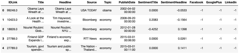

# Grab all the titles 
article_titles = main_data['Title']
# Create a list of strings, one for each title
titles_list = [title for title in article_titles]

# Collapse the list of strings into a single long string for processing
big_title_string = ' '.join(titles_list)

from nltk.tokenize import word_tokenize

# Tokenize the string into words
tokens = word_tokenize(big_title_string)

# Remove non-alphabetic tokens, such as punctuation
words = [word.lower() for word in tokens if word.isalpha()]

# Filter out stopwords
from nltk.corpus import stopwords
stop_words = set(stopwords.words('english'))

words = [word for word in words if not word in stop_words]

# Print first 10 words
words[:10]

接下來，我們需要載入預訓練的word2vec模型。你可以在這裡找到幾個這樣的模型。由於這是一個新聞數據集，我使用的是谷歌新聞模型，該模型經過大約1000億字的培訓（哇）。

# Load word2vec model (trained on an enormous Google corpus)
model = gensim.models.KeyedVectors.load_word2vec_format('GoogleNews-vectors-negative300.bin', binary = True) 

# Check dimension of word vectors
model.vector_size

因此，模型將生成300維單詞向量，而我們創建向量所需要做的就是將其傳遞給模型。每個向量看起來像這樣：

economy_vec = model['economy']
economy_vec[:20] # First 20 components

word2vec（可以理解）不能從一個不在其辭彙表中的單詞創建一個向量。因此，我們需要在創建單詞向量的完整列表時指定「if model in model.vocab」。

# Filter the list of vectors to include only those that Word2Vec has a vector for
vector_list = [model[word] for word in words if word in model.vocab]

# Create a list of the words corresponding to these vectors
words_filtered = [word for word in words if word in model.vocab]

# Zip the words together with their vector representations
word_vec_zip = zip(words_filtered, vector_list)

# Cast to a dict so we can turn it into a DataFrame
word_vec_dict = dict(word_vec_zip)
df = pd.DataFrame.from_dict(word_vec_dict, orient='index')
df.head(3)

使用t-SNE降低維數

接下來，我們將使用t-SNE壓縮這些單詞向量（讀取：做降維），以查看是否出現任何模式。如果您不熟悉t-SNE及其解釋，請查看這篇關於t-SNE的優秀互動性distill.pub文章。

使用t-SNE的參數非常重要，因為不同的值會產生非常不同的結果。我測試了0到100之間的幾個值的困惑，並發現它每次產生大致相同的形狀。我測試了20到400之間的幾個學習率，並決定將學習率保持在默認值（200）。

為了可見性（和處理時間），我使用了400個單詞向量而不是大約20,000個左右。

from sklearn.manifold import TSNE

# Initialize t-SNE
tsne = TSNE(n_components = 2, init = 'random', random_state = 10, perplexity = 100)

# Use only 400 rows to shorten processing time
tsne_df = tsne.fit_transform(df[:400])

現在我們準備繪製減少的單詞向量數組。我曾經adjust_text智能地將文字分開，以提高可讀性：

sns.set()
# Initialize figure
fig, ax = plt.subplots(figsize = (11.7, 8.27))
sns.scatterplot(tsne_df[:, 0], tsne_df[:, 1], alpha = 0.5)

# Import adjustText, initialize list of texts
from adjustText import adjust_text
texts = []
words_to_plot = list(np.arange(0, 400, 10))

# Append words to list
for word in words_to_plot:
    texts.append(plt.text(tsne_df[word, 0], tsne_df[word, 1], df.index[word], fontsize = 14))
    
# Plot text using adjust_text (because overlapping text is hard to read)
adjust_text(texts, force_points = 0.4, force_text = 0.4, 
            expand_points = (2,1), expand_text = (1,2),
            arrowprops = dict(arrowstyle = "-", color = 'black', lw = 0.5))

plt.show()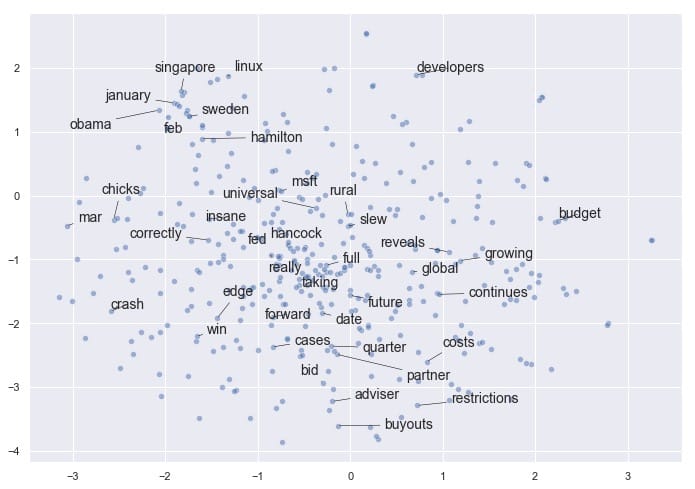

如果您有興趣嘗試adjust_text自己的繪圖需求，可以在這裡找到它。請務必使用camelcase導入它adjustText，請注意adjustText目前與matplotlib3.0或更高版本不兼容。

令人鼓舞的是，即使將矢量嵌入減少到2維，我們也會看到某些項聚集在一起。例如，我們在左/左上角有幾個月，我們的企業融資條件接近底部，我們在中間有更多通用的非主題詞（如「完整」，「真實」，「迴轉」）。

請注意，如果我們使用不同的參數再次運行t-SNE，我們可能會發現這個結果有一些相似之處，但我們不能保證看到完全相同的模式。t-SNE不是確定性的。相關地，簇的緊密度和簇之間的距離並不總是有意義的。它主要是作為一種探索性工具，而不是相似性的決定性指標。

平均詞嵌入

我們已經了解了嵌入文字如何應用於此數據集。現在我們可以繼續討論一些更有趣的ML應用程序：找到聚集在一起的標題，並查看出現的模式。

我們可以使用更簡單（有時甚至更有效）的技巧，而不是使用沒有預訓練模型的Doc2Vec，因此需要更長的訓練過程：平均每個文檔中單詞向量的嵌入。在我們的例子中，文檔是指標題。

我們需要重做預處理步驟以保持標題完整 – 正如我們將看到的，這比分裂單詞更複雜。值得慶幸的是，Dimitris Spathis 創建了一系列功能，我發現這些功能可以完美地用於這個精確的用例。謝謝，迪米特里斯！

def document_vector(word2vec_model, doc):
    # remove out-of-vocabulary words
    doc = [word for word in doc if word in model.vocab]
    return np.mean(model[doc], axis=0)

# Our earlier preprocessing was done when we were dealing only with word vectors
# Here, we need each document to remain a document 
def preprocess(text):
    text = text.lower()
    doc = word_tokenize(text)
    doc = [word for word in doc if word not in stop_words]
    doc = [word for word in doc if word.isalpha()] 
    return doc

# Function that will help us drop documents that have no word vectors in word2vec
def has_vector_representation(word2vec_model, doc):
    """check if at least one word of the document is in the
    word2vec dictionary"""
    return not all(word not in word2vec_model.vocab for word in doc)

# Filter out documents
def filter_docs(corpus, texts, condition_on_doc):
    """
    Filter corpus and texts given the function condition_on_doc which takes a doc. The document doc is kept if condition_on_doc(doc) is true.
    """
    number_of_docs = len(corpus)

    if texts is not None:
        texts = [text for (text, doc) in zip(texts, corpus)
                 if condition_on_doc(doc)]

    corpus = [doc for doc in corpus if condition_on_doc(doc)]

    print("{} docs removed".format(number_of_docs - len(corpus)))

    return (corpus, texts)

現在我們將使用它們來進行處理：

# Preprocess the corpus
corpus = [preprocess(title) for title in titles_list]

# Remove docs that don't include any words in W2V's vocab
corpus, titles_list = filter_docs(corpus, titles_list, lambda doc: has_vector_representation(model, doc))

# Filter out any empty docs
corpus, titles_list = filter_docs(corpus, titles_list, lambda doc: (len(doc) != 0))
x = []
for doc in corpus: # append the vector for each document
    x.append(document_vector(model, doc))
    
X = np.array(x) # list to array

t-SNE，第2輪：文件向量

現在我們已經成功創建了我們的文檔向量數組，讓我們看看在使用t-SNE繪製它們時是否可以獲得類似的有趣結果。

# Initialize t-SNE
tsne = TSNE(n_components = 2, init = 'random', random_state = 10, perplexity = 100)

# Again use only 400 rows to shorten processing time
tsne_df = tsne.fit_transform(X[:400])
fig, ax = plt.subplots(figsize = (14, 10))
sns.scatterplot(tsne_df[:, 0], tsne_df[:, 1], alpha = 0.5)

from adjustText import adjust_text
texts = []
titles_to_plot = list(np.arange(0, 400, 40)) # plots every 40th title in first 400 titles

# Append words to list
for title in titles_to_plot:
    texts.append(plt.text(tsne_df[title, 0], tsne_df[title, 1], titles_list[title], fontsize = 14))
    
# Plot text using adjust_text
adjust_text(texts, force_points = 0.4, force_text = 0.4, 
            expand_points = (2,1), expand_text = (1,2),
            arrowprops = dict(arrowstyle = "-", color = 'black', lw = 0.5))

plt.show()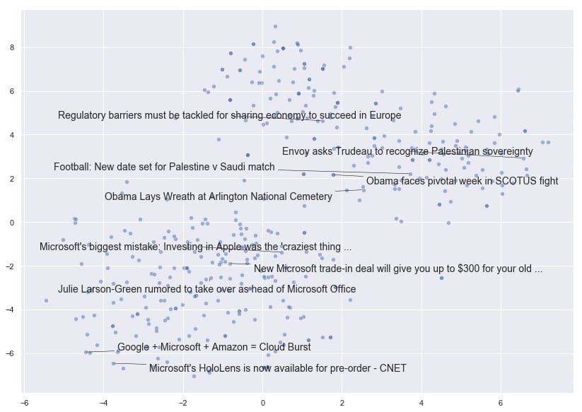

非常有趣！我們可以看到t-SNE已經將文檔向量摺疊成一個維度空間，文檔根據其內容是否與國家，世界領導者和外交事務有關，或者與技術公司有更多關係而展開。

現在讓我們探討文章的受歡迎程度。共識認為，文章標題越聳人聽聞或點擊率越高，分享的可能性越大，對吧？接下來，我們將看看在這個特定的數據集中是否有證據表明。

人氣和情感分析

首先，我們需要刪除所有沒有受歡迎度測量或來源的文章。用於流行度的空測量在該數據中表示為-1。

# Drop all the rows where the article popularities are unknown (this is only about 11% of the data)
main_data = main_data.drop(main_data[(main_data.Facebook == -1) | 
                                     (main_data.GooglePlus == -1) | 
                                     (main_data.LinkedIn == -1)].index)

# Also drop all rows where we don't know the source
main_data = main_data.drop(main_data[main_data['Source'].isna()].index)

main_data.shape

我們仍然有81,000篇文章可供使用，所以讓我們看看我們是否能找到情緒和股票數量之間的關聯。

fig, ax = plt.subplots(1, 3, figsize=(15, 10))

subplots = [a for a in ax]
platforms = ['Facebook', 'GooglePlus', 'LinkedIn']
colors = list(sns.husl_palette(10, h=.5)[1:4]) 

for platform, subplot, color in zip(platforms, subplots, colors):
    sns.scatterplot(x = main_data[platform], y = main_data['SentimentTitle'], ax=subplot, color=color)
    subplot.set_title(platform, fontsize=18)
    subplot.set_xlabel('') 
    
fig.suptitle('Plot of Popularity (Shares) by Title Sentiment', fontsize=24)

plt.show()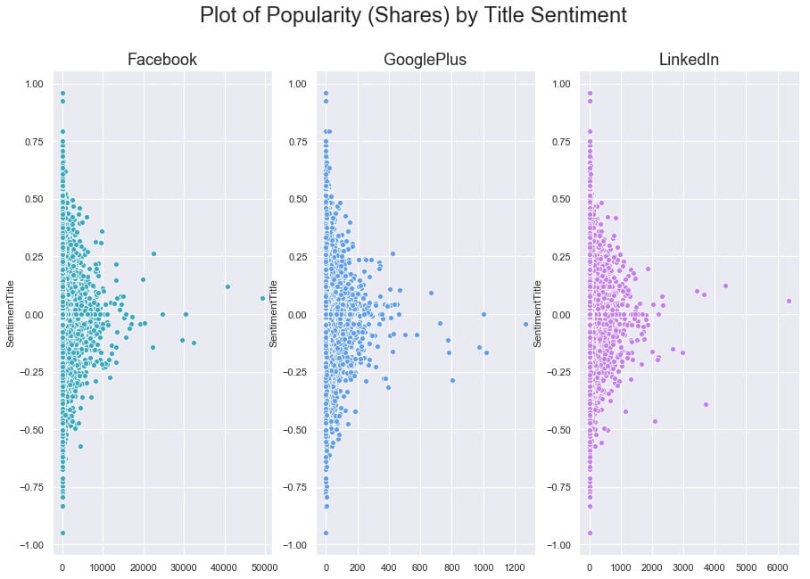

要弄清楚這裡是否存在任何關係有點困難，因為一些文章在其份額方面是重要的異常值。讓我們嘗試對x軸進行對數轉換，看看我們是否可以揭示任何模式。我們還將使用regplot，因此seaborn將覆蓋每個圖的線性回歸。

# Our data has over 80,000 rows, so let's also subsample it to make the log-transformed scatterplot easier to read

subsample = main_data.sample(5000)

fig, ax = plt.subplots(1, 3, figsize=(15, 10))

subplots = [a for a in ax]

for platform, subplot, color in zip(platforms, subplots, colors):
    # Regression plot, so we can gauge the linear relationship
    sns.regplot(x = np.log(subsample[platform] + 1), y = subsample['SentimentTitle'], 
                ax=subplot, 
                color=color,
                # Pass an alpha value to regplot's scatterplot call
                scatter_kws={'alpha':0.5})
    
    # Set a nice title, get rid of x labels
    subplot.set_title(platform, fontsize=18)
    subplot.set_xlabel('') 
    
fig.suptitle('Plot of log(Popularity) by Title Sentiment', fontsize=24)

plt.show()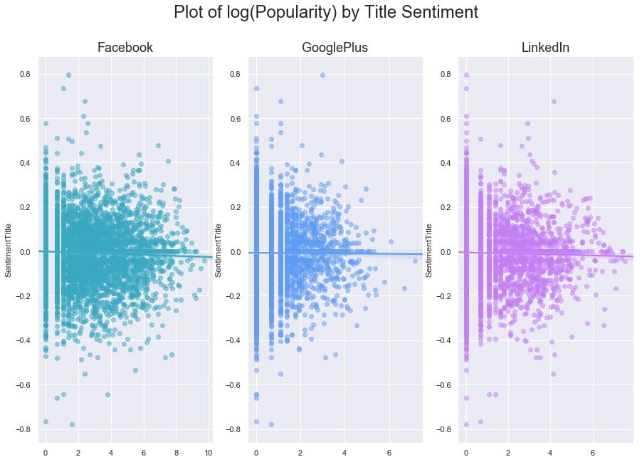

與我們可能期望的相反（來自我們對高度情緒化，點擊率標題的看法），在這個數據集中，我們發現標題情緒與通過股票數量衡量的文章受歡迎程度之間沒有關係。

為了更清楚地了解受歡迎程度如何看待自己，讓我們按平台製作最終的日誌（人氣）。

fig, ax = plt.subplots(3, 1, figsize=(15, 10))

subplots = [a for a in ax]

for platform, subplot, color in zip(platforms, subplots, colors):
  
    sns.distplot(np.log(main_data[platform] + 1), ax=subplot, color=color, kde_kws={'shade':True})
    
    # Set a nice title, get rid of x labels
    subplot.set_title(platform, fontsize=18)
    subplot.set_xlabel('') 
    
fig.suptitle('Plot of Popularity by Platform', fontsize=24)

plt.show()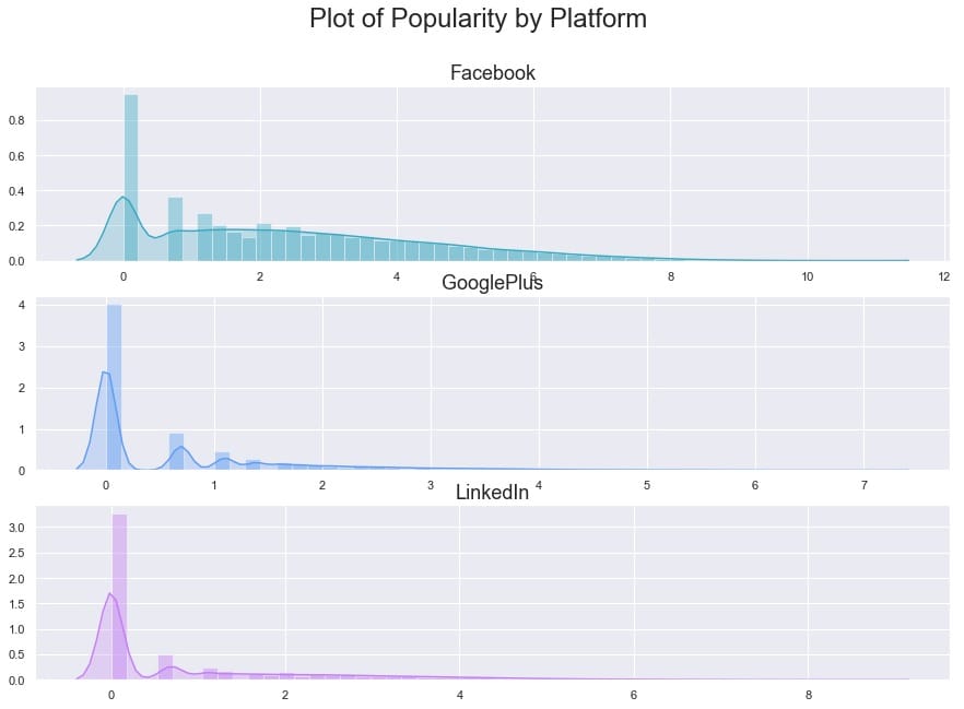

作為我們最後的探索部分，讓我們來看看情緒本身。出版商之間似乎有所不同嗎？

# Get the list of top 12 sources by number of articles
source_names = list(main_data['Source'].value_counts()[:12].index)
source_colors = list(sns.husl_palette(12, h=.5))

fig, ax = plt.subplots(4, 3, figsize=(20, 15), sharex=True, sharey=True)

ax = ax.flatten()
for ax, source, color in zip(ax, source_names, source_colors):
    sns.distplot(main_data.loc[main_data['Source'] == source]['SentimentTitle'],
                               ax=ax, color=color, kde_kws={'shade':True})
    ax.set_title(source, fontsize=14)
    ax.set_xlabel('')
    
plt.xlim(-0.75, 0.75)
plt.show()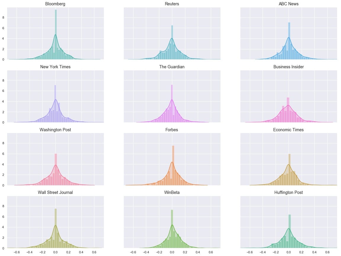

的分布看起來非常相似，但它是一個有點很難說如何相似時，他們都在不同的地塊。讓我們嘗試將它們全部疊加在一個圖上。

# Overlay each density curve on the same plot for closer comparison

fig, ax = plt.subplots(figsize=(12, 8))

for source, color in zip(source_names, source_colors):
    sns.distplot(main_data.loc[main_data['Source'] == source]['SentimentTitle'],
                               ax=ax, hist=False, label=source, color=color)
    ax.set_xlabel('')
    
plt.xlim(-0.75, 0.75)
plt.show()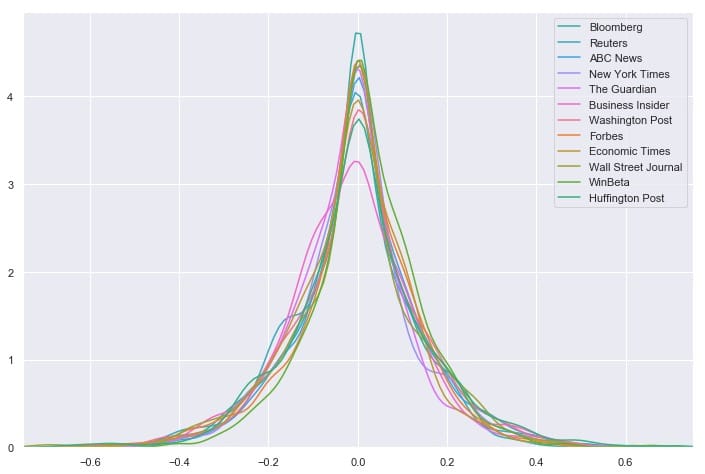

我們看到消息來源對文章標題的情感分布非常相似 – 看起來任何一個來源都不是正面或負面標題的異常值。相反，所有12個最常見的源都具有以0為中心的分布，具有適度大小的尾部。但是這能說出完整的故事嗎？讓我們再看一下這些數字：

# Group by Source, then get descriptive statistics for title sentiment
source_info = main_data.groupby('Source')['SentimentTitle'].describe()
# Recall that `source_names` contains the top 12 sources
# We'll also sort by highest standard deviation
source_info.loc[source_names].sort_values('std', ascending=False)[['std', 'min', 'max']]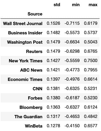

我們可以一眼看出，華爾街日報的標準差最大，範圍最大，與其他任何頂級資源相比，最低情緒最低。這表明華爾街日報在文章標題方面可能異常負面。要嚴格驗證這一點需要進行假設檢驗，這超出了本文的範圍，但這是一個有趣的潛在發現和未來方向。

人氣預測

我們為建模數據準備的第一個任務是重新加入帶有各自標題的文檔向量。值得慶幸的是，當我們在預處理語料，我們處理corpus和titles_list同步，所以他們所代表的載體和標題仍將匹配。與此同時，main_df我們已經刪除了所有具有-1流行度的文章，因此我們需要刪除代表這些文章標題的向量。

在這台計算機上不可能對這些巨大的載體進行模型訓練，但我們會看到通過減少一點維度可以做些什麼。我還將根據發布日期設計一個新功能：「DaysSinceEpoch」，它基於Unix時間（在此處閱讀更多內容）。

import datetime

# Convert publish date column to make it compatible with other datetime objects

main_data['PublishDate'] = pd.to_datetime(main_data['PublishDate'])

# Time since Linux Epoch
t = datetime.datetime(1970, 1, 1)

# Subtract this time from each article's publish date
main_data['TimeSinceEpoch'] = main_data['PublishDate'] - t

# Create another column for just the days from the timedelta objects 
main_data['DaysSinceEpoch'] = main_data['TimeSinceEpoch'].astype('timedelta64[D]')

main_data['TimeSinceEpoch'].describe()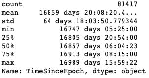

正如我們所看到的，所有這些文章都是在彼此約250天內發布的。

from sklearn.decomposition import PCA

pca = PCA(n_components=15, random_state=10)

# as a reminder, x is the array with our 300-dimensional vectors
reduced_vecs = pca.fit_transform(x)
df_w_vectors = pd.DataFrame(reduced_vecs)

df_w_vectors['Title'] = titles_list
# Use pd.concat to match original titles with their vectors
main_w_vectors = pd.concat((df_w_vectors, main_data), axis=1)

# Get rid of vectors that couldn't be matched with the main_df
main_w_vectors.dropna(axis=0, inplace=True)

現在我們需要刪除非數字和非虛擬列，以便我們可以將數據提供給模型。我們還將對該DaysSinceEpoch特徵應用縮放，因為與減少的單詞向量，情緒等相比，它的幅度要大得多。

# Drop all non-numeric, non-dummy columns, for feeding into the models
cols_to_drop = ['IDLink', 'Title', 'TimeSinceEpoch', 'Headline', 'PublishDate', 'Source'] 

data_only_df = pd.get_dummies(main_w_vectors, columns = ['Topic']).drop(columns=cols_to_drop)

# Standardize DaysSinceEpoch since the raw numbers are larger in magnitude 
from sklearn.preprocessing import StandardScaler

scaler = StandardScaler()

# Reshape so we can feed the column to the scaler
standardized_days = np.array(data_only_df['DaysSinceEpoch']).reshape(-1, 1)
data_only_df['StandardizedDays'] = scaler.fit_transform(standardized_days)

# Drop the raw column; we don't need it anymore
data_only_df.drop(columns=['DaysSinceEpoch'], inplace=True)

# Look at the new range
data_only_df['StandardizedDays'].describe()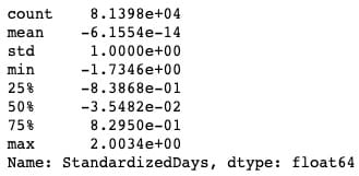

# Get Facebook data only
fb_data_only_df = data_only_df.drop(columns=['GooglePlus', 'LinkedIn'])
# Separate the features and the response
X = fb_data_only_df.drop('Facebook', axis=1)
y = fb_data_only_df['Facebook']

# 80% of data goes to training
X_train, X_test, y_train, y_test = train_test_split(X, y, test_size = 0.2, random_state = 10)

讓我們XGBoost對數據進行非優化，看看它是如何開箱即用的。

from sklearn.metrics import mean_squared_error

# Instantiate an XGBRegressor
xgr = xgb.XGBRegressor(random_state=2)

# Fit the classifier to the training set
xgr.fit(X_train, y_train)

y_pred = xgr.predict(X_test)

mean_squared_error(y_test, y_pred)

至少可以說，結果並不令人滿意。我們可以通過超參數調整來改善這種性能嗎？我已經從這篇Kaggle文章中提取並重新調整了一個超參數調整網格。

from sklearn.model_selection import GridSearchCV

# Various hyper-parameters to tune
xgb1 = xgb.XGBRegressor()
parameters = {'nthread':[4], 
              'objective':['reg:linear'],
              'learning_rate': [.03, 0.05, .07], 
              'max_depth': [5, 6, 7],
              'min_child_weight': [4],
              'silent': [1],
              'subsample': [0.7],
              'colsample_bytree': [0.7],
              'n_estimators': [250]}

xgb_grid = GridSearchCV(xgb1,
                        parameters,
                        cv = 2,
                        n_jobs = 5,
                        verbose=True)

xgb_grid.fit(X_train, y_train)

據xgb_grid我們所知，我們的最佳參數如下：

{'colsample_bytree'：0.7，'learning_rate'：0.03，'max_depth'：5，'min_child_weight'：4，'n_estimators'：250，'nthread'：4，'objective'：'reg：linear'，'silent' ：1，'subsample'：0.7}

使用新參數再試一次：

params = {'colsample_bytree': 0.7, 'learning_rate': 0.03, 'max_depth': 5, 'min_child_weight': 4, 
          'n_estimators': 250, 'nthread': 4, 'objective': 'reg:linear', 'silent': 1, 'subsample': 0.7}

# Try again with new params
xgr = xgb.XGBRegressor(random_state=2, **params)

# Fit the classifier to the training set
xgr.fit(X_train, y_train)

y_pred = xgr.predict(X_test)

mean_squared_error(y_test, y_pred)

它大約35,000更好，但我不確定是說了很多。在這一點上，我們可能推斷出當前狀態下的數據似乎不足以使該模型執行。讓我們看看我們是否可以通過更多的特徵工程來改進它：我們將訓練一些分類器來分離兩組主要文章：Duds（0或1份）與Not Duds。

我們的想法是，如果我們能給回歸量一個新的特徵（該文章具有極低的份額的可能性），它可能更有利於預測高度共享的文章，從而降低這些文章的殘值並減少均方。錯誤。

繞道：檢測無用品

從我們之前製作的對數轉換圖中，我們可以注意到，一般來說，有2個文章塊：1個簇在0，另一個簇（長尾）從1開始。我們可以訓練一些分類器來識別文章是否是「啞彈」（在0-1股票箱中），然後使用這些模型的預測作為最終回歸量的特徵，這將預測概率。這稱為模型堆疊。

# Define a quick function that will return 1 (true) if the article has 0-1 share(s)
def dud_finder(popularity):
    if popularity <= 1:
        return 1
    else:
        return 0
# Create target column using the function
fb_data_only_df['is_dud'] = fb_data_only_df['Facebook'].apply(dud_finder)
fb_data_only_df[['Facebook', 'is_dud']].head()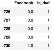

# 28% of articles can be classified as "duds"
fb_data_only_df['is_dud'].sum() / len(fb_data_only_df)

現在我們已經完成了dud功能，我們將初始化分類器。我們將使用隨機森林，優化的XGBC分類器和K-Nearest Neighbors分類器。我將省略調整XGB的部分，因為它看起來與我們之前做的調整基本相同。

from sklearn.ensemble import RandomForestClassifier
from sklearn.neighbors import KNeighborsClassifier
from sklearn.model_selection import train_test_split
X = fb_data_only_df.drop(['is_dud', 'Facebook'], axis=1)
y = fb_data_only_df['is_dud']
# 80% of data goes to training
X_train, X_test, y_train, y_test = train_test_split(X, y, test_size = 0.2, random_state = 10)
# Best params, produced by HP tuning
params = {'colsample_bytree': 0.7, 'learning_rate': 0.03, 'max_depth': 5, 'min_child_weight': 4, 
          'n_estimators': 200, 'nthread': 4, 'silent': 1, 'subsample': 0.7}
# Try xgc again with new params
xgc = xgb.XGBClassifier(random_state=10, **params)
rfc = RandomForestClassifier(n_estimators=100, random_state=10)
knn = KNeighborsClassifier()
preds = {}
for model_name, model in zip(['XGClassifier', 'RandomForestClassifier', 'KNearestNeighbors'], [xgc, rfc, knn]):
    model.fit(X_train, y_train)
    preds[model_name] = model.predict(X_test)

測試模型，獲取分類報告：

from sklearn.metrics import classification_report, roc_curve, roc_auc_score
for k in preds:
    print("{} performance:".format(k))
    print()
    print(classification_report(y_test, preds[k]), sep='\n')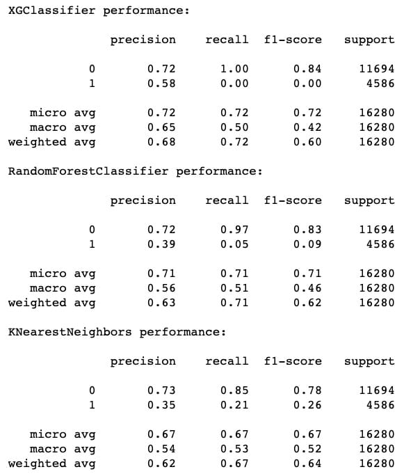

f1-score的最高表現來自XGC，其次是RF，最後是KNN。但是，我們也可以注意到，KNN 在召回方面確實做得最好（成功識別啞彈）。這就是為什麼模型堆疊是有價值的 – 有時甚至像XGBoost這樣的優秀模型也會在像這樣的任務上表現不佳，顯然要識別的功能可以在本地近似。包括KNN的預測應該增加一些急需的多樣性。

# Plot ROC curves
for model in [xgc, rfc, knn]:
    fpr, tpr, thresholds = roc_curve(y_test, model.predict_proba(X_test)[:,1])
    plt.plot([0, 1], [0, 1], 'k--')
    plt.plot(fpr, tpr)
    
plt.xlabel('False Positive Rate')
plt.ylabel('True Positive Rate')
plt.title('ROC Curves')
plt.show()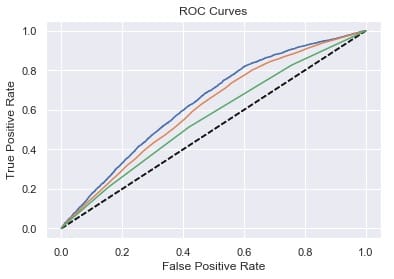

人氣預測：第2輪

現在我們可以從三個分類器中平均出概率預測，並將其用作回歸量的特徵。

averaged_probs =（xgc.predict_proba（X）[：，1] + 
                  knn.predict_proba（X）[：，1] + 
                  rfc.predict_proba（X）[：，1]）/ 3
X ['prob_dud'] = averaged_probs 
y = fb_data_only_df ['Facebook']

接下來是另一輪惠普調整，包括新功能，我將遺漏。讓我們看看我們如何處理性能：

xgr = xgb.XGBRegressor(random_state=2, **params)
# Fit the classifier to the training set
xgr.fit(X_train, y_train)
y_pred = xgr.predict(X_test)
mean_squared_error(y_test, y_pred)

哦哦！這種性能與我們甚至進行任何模型堆疊之前的性能基本相同。也就是說，我們可以記住，MSE作為誤差測量傾向於超重異常值。實際上，我們還可以計算平均絕對誤差（MAE），用於評估具有顯著異常值的數據的性能。在數學術語中，MAE計算殘差的l1範數，基本上是絕對值，而不是MSE使用的l2範數。我們可以將MAE與MSE的平方根進行比較，也稱為均方根誤差（RMSE）。

mean_absolute_error（y_test，y_pred），np.sqrt（mean_squared_error（y_test，y_pred））

平均絕對誤差僅為RMSE的1/3左右！也許我們的模型並不像我們最初想的那麼糟糕。

最後一步，讓我們根據XGRegressor了解每個功能的重要性：

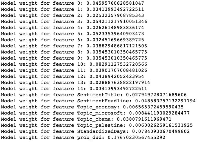
整齊！我們的模型被發現prob_dud是最重要的功能，我們的自定義StandardizedDays功能是第二重要的功能。（特徵0到14對應於縮小的標題嵌入向量。）

儘管通過這一輪模型堆疊沒有改善整體性能，但我們可以看到我們成功地捕獲了數據的一個重要變異來源，模型已經開始了。

如果我要繼續擴展這個項目以使模型更準確，我可能會考慮使用外部數據來增加數據，包括通過分箱或散列將Source作為變數，在原始300維向量上運行模型，以及使用每個文章在不同時間點的流行度的「時間分片」數據（該數據的伴隨數據集）來預測最終流行度。

如果您發現此分析很有趣，請隨時使用該代碼，並進一步擴展它！筆記本在這裡（請注意，某些單元格的順序可能與此處顯示的順序略有不同），此項目使用的原始數據在此處。